
Can Heat From Below Explain the Abyssal Warming Acceleration?
I’ve been working through whether geothermal or hydrothermal heat could explain the warming acceleration in the abyssal ocean. This one’s taken a lot longer than I expected, mostly because I need it to work quantitatively.
There’s definitely heat coming out of the Earth. That part isn’t controversial. But, it has to be enough heat. It has to show up in the right places. It should make sense with the vertical structure of the warming. And, most importantly, it has to explain why the warming rate itself is increasing.
That last part changes the whole problem.
I’m not just testing warming
The signal I’m trying to explain is a warming acceleration. So, I’m not only asking whether temperature is going up. I’m asking whether the rate of warming is also going up. The heat needs to satisfy this equation:
Here, the temperature changes over time, but the important term for me is the acceleration, a. The warming rate is:
And the warming acceleration is:
A constant geothermal heat source can warm the ocean, but a constant heat source doesn’t automatically explain why the warming rate is increasing. For that, something has to change. Either the geothermal source itself has to increase (already tested)...or the ocean has to start moving more of that heat into the warming region. That second possibility is the one I’m still testing.
How much extra heat does the acceleration require?
The first thing I did was convert the observed temperature acceleration into an energy requirement. The basic heat equation is:
So, if temperature is accelerating, the required heating rate is accelerating, too. That becomes:
For the positive abyssal warming acceleration footprint, I get a required increase in heating rate of about:
By the end of the analysis period, that builds to about:
≈ 8.3 terawatts
And, the total energy burden over the interval is about:,
So, that gave me a pretty clear target. If geothermal heat is going to explain the acceleration, somehow it has to account for that growing heat requirement.
I built three different geothermal source maps
I didn’t want to use one single number for geothermal heat, because there are different ways to estimate it. I also wanted to understand the uncertainty and error of that value. So, I tested three different source fields. The first is ordinary conductive heat flow through the seafloor. Globally, that comes out to about:
Second, I used a more generous lithospheric heat loss estimate based largely on crustal age. That gives:
I treat that as more of an upper bound. Finally, I estimated a hydrothermal residual by subtracting the conductive part from the broader lithospheric heat loss estimate: That gives roughly:
I kept these separate as three different estimates of geothermal heat.
The energy test already made geothermal harder
If I only count the geothermal heat available beneath the parts of the abyssal ocean that are actually showing positive warming acceleration, how much of the required heating could it supply?
The approximate ratios came out to:
Total lithospheric estimate: ~0.33
Hydrothermal residual: ~0.08
The conductive estimate supplied about 25% of the required power. The lithospheric estimate got us to about 33%, and the hydrothermal residual was only about 8%. So,
So, we aren’t quite getting enough geothermal power underneath the warming footprint, yet magnitude alone isn’t enough to close it.
A source can be smaller globally and still be the dominant source if circulation focuses it into the right places. So, I kept going…
Does the warming happen where the geothermal heat is?
This was the next obvious test. If geothermal heating is driving the abyssal acceleration, I’d expect at least some relationship between the warming pattern and things like:
high seafloor heat flow
young ocean crust
mid ocean ridges
known hydrothermal vents
broader hydrothermal source regions
So, I compared the observed warming acceleration with the geothermal source maps and tried to find a correlation. And, the correlations were tiny. For the three main source fields, I got values around:
Lithospheric: r ≈ 0.026
Hydrothermal residual: r ≈ 0.019
I also used geographically blocked tests and leave one basin out tests. Those relationships didn’t hold up. That doesn’t mean there aren’t undiscovered vents. There probably are. It just means the large scale abyssal warming pattern isn’t strongly following the geothermal source pattern I can actually test.
The centroid put the warming deep. But is it actually bottom intensified?
Earlier in this project, I also went back and re-constructed Roger Cunningham’s (@TheEthicalSkeptic) 4,413 m centroid calculation (see Figure 1) to see how robust it was to perterbations. His estimate was based on the vertical distribution of deep and abyssal warming reported by Desbruyères et al. [1]. I reconstructed the calculation independently, and then repeated the centroid calculation using the newer Johnson abyssal warming data [2]. Both put the center of the signal at roughly 4.41 km depth, so Roger’s original result turned out to be pretty robust.
That tells me the warming really is concentrated very deep in the ocean. But it still doesn’t tell me whether the warming is actually hugging the seafloor. A signal centered at 4.41 km could be right near the bottom in one basin and hundreds or even thousands of meters above it somewhere else. Since geothermal heat enters through the seafloor, I needed to test that more directly. So instead of measuring depth down from the surface, I measured the warming by height above the actual seafloor.
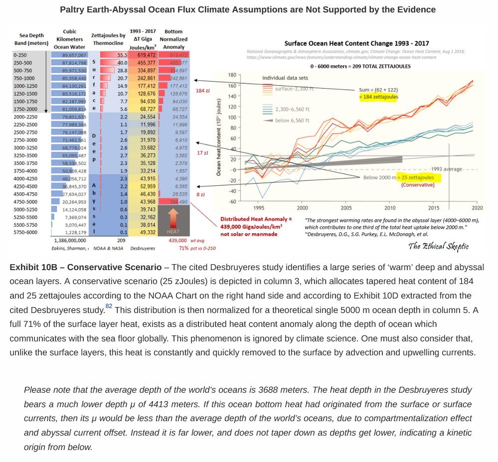
Figure 1. Roger’s reconstruction of the ocean heat content profile reported by Desbruyeres et al [1] ( Exhibit 10B ), which places the heat weighted vertical centroid at approximately 4,413 m depth. I later reconstructed this centroid independently from Johnson’s [2] underlying abyssal warming data and obtained essentially the same result. Source: Roger Cunningham / @TheEthicalSkeptic (Twitter)
If heat is coming through the seafloor, I’d expect the signal to get stronger as I get closer to the seafloor. So, instead of only looking at fixed pressure layers, I followed the shape of the bottom. I compared water close to the seafloor with water above it. ,Roughly:
0–500 m above bottom
500–2000 m above bottom
Then, I calculated:
If there’s strong bottom intensified geothermal heating, I’d expect:
But instead, I got:
So, the layer closest to the bottom actually had a smaller acceleration in that comparison. And, the thing I was looking for … clear positive bottom intensification, wasn’t there.
Also, the sign stayed negative when I repeated the test while leaving out individual ocean basins. Pretty robust.
Then I looked at temperature and salinity together
Heating changes temperature AND density. Density depends on both temperature and salinity.
The first term is thermal, the second is salinity. For plain conductive geothermal heating, the basic expectation is that the seafloor adds heat, not salt. So, near the source I’d expect the thermal part to matter more.
Hydrothermal systems are messier because vent fluids can be saltier or fresher depending on what’s happening below the seafloor. So, I didn’t assume hydrothermal plumes should always have one particular salinity sign. Instead, I investigated whether the abyssal changes become more thermally dominated near the bottom.
They didn’t.
I also looked at temperature and salinity together while following the same density surfaces. On those surfaces, temperature and salinity changes were almost always offsetting each other:
This means, when the water got warmer, the salinity usually changed in a way that helped keep the density similar. It’s not really a geothermal fingerprint by itself, and what I really wanted to know was whether the temperature part became more important as I got closer to the seafloor. If heat is being added from below, I’d expect a stronger thermal signal near the bottom.
I didn’t see that.
So the useful result here was that the changes didn’t become more thermally dominated near the seafloor, which is what I would’ve expected from a simple geothermal heating picture.
What about individual hydrothermal plumes?
I tested that separately because vents are very different from slow, diffuse conductive heating.
Here I investigated whether a hydrothermal plume have enough power locally, could it rise far enough, could it reach the observed abyssal layers, and could enough plumes cover enough of the warming footprint.
The basic coverage calculation is:
The interesting thing is that power itself wasn’t the biggest problem. Individual hydrothermal systems can definitely produce strong local heating. And, vertical reach wasn’t a problem either.
With broad sensitivity assumptions, as much as:
But geographic coverage was much worse.
For the known vent test, I used the InterRidge Global Database of Active Submarine Hydrothermal Vent Fields, version 3.4, which was completed in 2020. It contains 721 catalogued vent fields: 304 confirmed active, 362 inferred active, and 55 classified as inactive. For this test I used the 666 confirmed or inferred active sites.
I treated this value as a lower bound, and did not assume that areas without a mapped vent have no hydrothermal activity. I also didn’t assume a plume had to stay right next to the vent. I tested lateral footprints around the vent locations:
So at the upper end, I was allowing a known vent to potentially affect abyssal targets as far as 500 km away. I also tested plume rise heights from 50 m all the way to 2,000 m, rather than assuming the heat stayed right at the seafloor. Even across that broad sensitivity range, the known active & inferred vent set only reached:
of the positive abyssal warming acceleration.
I then made the geographic test even more generous. Instead of requiring a plume to be near a vent we’ve actually discovered, I treated the global spreading ridge system as a broader hydrothermal opportunity region. For the wider geothermal analysis, I also used EarthByte’s 2020 present day oceanic crust age and seafloor spreading grids, which give me an independent map of where young crust and active spreading are located.
In the plume calculation, I tested ridge-source spacing of:
and allowed the active fraction of that ridge opportunity to range all the way up to an intentionally extreme 100% active case. Even then, the optimistic ridge-opportunity result only reached:
So, I tried to give the hydrothermal explanation a lot more room than the dataset gives us. The problem was that even with very large plume footprints and a much broader ridge opportunity test, it still didn’t reach much of the observed positive abyssal warming burden. So, hydrothermal plumes can definitely matter locally, but even when I allow a lot of flexibility in their location, they don’t cover much of the large scale abyssal warming signal. That’s why my current classification is:
energetically possible locally, but coverage insufficient as the dominant explanation.
The timing problem
The geothermal source maps I’m using are basically static. So, if the source power is constant:
That makes it challenging to directly create a warming acceleration. But, there’s another possibility. Maybe the source stays constant while the fraction of that heat delivered into the abyssal warming region changes. If the delivered geothermal power is:
then for a constant geothermal source:
So, the source itself doesn’t have to change. The ocean could change where the heat goes. That’s the last major geothermal loophole I’m testing. The required change in delivered fraction is pretty big. For the three source estimates, I calculated:
Lithospheric/GDH1: Δf ≈ 0.288
Hydrothermal residual: Δf ≈ 0.683
So, depending on which source estimate I use, circulation would need to change the delivered fraction by roughly:
That’s a lot, but still possible.
That’s why I downloaded about 20 years of 3D ocean circulation data
This is the part that turned into a whole numerical modeling project. I downloaded monthly ORAS5 3D ocean velocity fields from:
240 months
The idea is to put a virtual geothermal heat tag into the bottom of the ocean model and let the currents move it. For each wet ocean cell, I keep track of geothermal-origin heat:
Then I convert that to heat per unit volume:
If water crosses a model cell face with volume transport Q, the heat crossing that face is:
And, the cell gets updated like this:
That’s really all the tracer is doing. Heat enters through the bottom; water moves it around, and I keep track of where it goes…. simple, but very annoying grid. :)
The polar grid caused a problem
ORAS5 uses what’s called an ORCA tripolar grid. Near the North Pole, the grid folds back on itself instead of meeting at one normal pole. That works for ocean models, but it makes transferring another dataset onto the grid pretty easy to mess up. And, it did create a problem.
In one version of the conservative remapping, some geothermal source cells were being covered by as much as:
That’s obviously wrong, and it meant some physical areas near the fold were getting counted more than once. So, I stopped the calculation and traced it. The problem came from the raw polygon geometry at the northern fold.
I rebuilt 349 of those fold polygons using the already validated ORCA neighbor connections instead of trusting the bad raw corner geometry.
Now the basic physical requirement is:
This means the total destination area overlapping a source cell can’t be larger than the source cell itself. And, for a fully covered source cell:
That finally passed, and there are now:
0 destination cells above 100% coverage
within the numerical tolerance. So, the remapping problem is finally fixed.
Geothermal power now survives the grid transfer almost perfectly
Once the physical grid was fixed, I rebuilt the conservative geothermal mapping. For the conductive source, the amount of geothermal power that can actually be mapped onto the ORAS5 ocean grid is:
At this point the grid transfer is conserving the geothermal source very precisely, and this part is finally done.
What’s left?
Now, I need to actually move the heat. The full ORAS5 ocean has roughly:
The little reference version of my transport solver already passes the basic tests: it conserves the heat, it behaves correctly with no flow and with source only heating, it works on 1D and 3D test cases, it handles partial bottom cells, and it stays deterministic.
The problem is that the reference version isn’t built to run the whole global ocean efficiently. So, now I’m writing a compiled, memory safe version of exactly the same calculation. Before I trust it, it has to reproduce the simple reference solver.
Time step limit
I’m not allowing the solver to move too much heat out of a grid cell in a single step otherwise the calculation starts to become unstable. I’m controlling that with what’s called a Courant-Friedrichs-Lewy (CFL) condition:
This checks how much water is trying to leave each cell during one time step compared with how much water is actually in that cell. I’m keeping that value below:
For April 2004, that means the model can only step forward by about:
≈ 32.8 minutes
So, just getting through that one month takes roughly:
That’s why this part has become a huge computational problem. The physics itself is really simple: move the tagged geothermal heat with the ocean currents and keep track of where it goes. The hard part is doing that across the full 3D ocean, over and over, without doing anything that could make the solver unstable or accidentally create or lose heat.
Once that works, the final geothermal test is easy… conceptually
I’ll run two versions of the ocean.
Run 1: the actual changing circulation
This uses the real month by month ORAS5 circulation from 2004-2024.
Run 2: a repeating seasonal ocean
For this one, I’ll build an average January circulation, average February circulation, average March circulation, etc. Then, I repeat that same seasonal year over and over. Both runs get exactly the same:
geothermal source
starting heat distribution
ocean grid
transport solver
time step rules
The only difference is whether the long-term circulation changes are allowed. Then, I calculate:
That tells me how much changing circulation itself changed the delivery of geothermal heat. And, then I compare that with what the observations require.
The targets are:
GDH1: Δf ≈ 0.288
Hydrothermal residual: Δf ≈ 0.683
That’s the test that’ll finally tell me whether circulation can rescue the geothermal explanation. It’s running right now.
So where does geothermal stand right now?
At this point, the simple versions aren’t doing very well. The available conductive heat looks too small. The warming pattern doesn’t strongly follow the geothermal source maps. The abyssal acceleration doesn’t get stronger toward the seafloor the way I expected from a simple bottom heating picture. The temperature and salinity structure doesn’t show a clear bottom intensified geothermal fingerprint. Hydrothermal plumes can provide plenty of heat locally, but even optimistic assumptions only cover around 8.5% of the abyssal warming acceleration observation. And, I don’t have evidence that the geothermal source itself has increased enough over time to explain the acceleration directly.
So geothermal/hydrothermal heating is looking pretty weak as the dominant explanation. But, I’m not closing it yet! There’s still one real possibility left:
maybe the heat source stayed mostly constant, but abyssal circulation changed where that heat was going. That’s what I’m testing right now. The source maps are built, and the polar grid problem is fixed. The geothermal power now transfers onto the ocean grid with essentially no numerical loss. :) Now, I need to move that heat through the full 3D ocean without creating or destroying it.
Once that solver passes, I can finally run the actual redistribution test.
And then I should be able to say, quantitatively, whether geothermal/hydrothermal heating still has a path to explaining the abyssal warming acceleration...
or whether I can finally close this mechanism.
References
[1] Desbruyères, D. G., Purkey, S. G., McDonagh, E. L., Johnson, G. C., & King, B. A. (2016). Deep and abyssal ocean warming from 35 years of repeat hydrography.Geophysical Research Letters, 43, 10,356–10,365. doi:10.1002/2016GL070413. The paper found the strongest warming rates in the 4,000–6,000 m abyssal layer.
[2] Johnson, G. C. (2026). Observed Multi-Decadal Acceleration of Globally Averaged Abyssal Ocean Warming.Geophysical Research Letters. doi:10.1029/2026GL124104. Johnson found a statistically significant increase in the globally integrated abyssal heat-uptake rate, from about 5.4 TW in 1988 to 20.2 TW in 2018.
